HelloWorld

Towards Practical Applications of Generative Driving World Models

Multimodal Video + LiDAR
Multi-view
Strong Pose Control
Layout Control 3D Boxes + Maps + Traffic Lights
Causal DiT

HelloWorld Team

Technical Report · Coming soon Explore applications

HelloWorld as a Data Generalizer

Edit a driving scene to generate controllable, multi-modal training data.

HelloWorld as a Closed-Loop Simulator

Recorded driving on the left and an Alpamayo 1.5 closed-loop rollout in HelloWorld on the right. The policy follows a slow-moving lead vehicle and adjusts its gap while a stopped vehicle in the right lane limits an immediate merge.

Model Overview

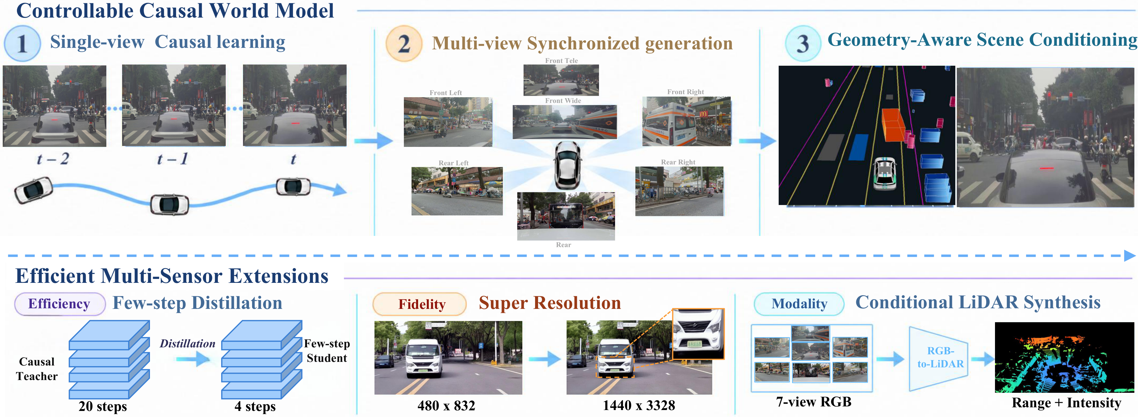
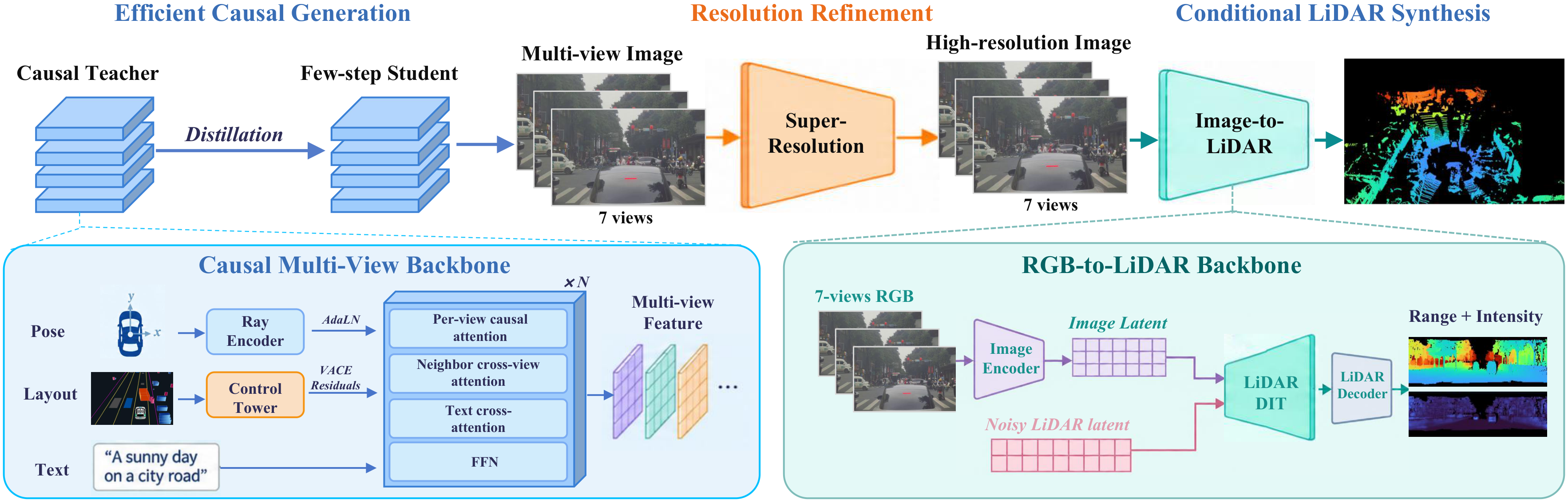
HelloWorld combines controllable multi-view video generation, few-step inference, super-resolution, and RGB-conditioned LiDAR synthesis in a unified driving world model system.

HelloWorld overview: single-view causal learning, synchronized multi-view generation, geometry-aware scene conditioning, and efficient multi-sensor extensions. — Controllable causal generation with few-step distillation, super-resolution, and conditional LiDAR synthesis.

HelloWorld architecture: causal multi-view backbone, few-step distillation, super-resolution, and RGB-to-LiDAR backbone. — Causal multi-view generation, few-step distillation, super-resolution, and RGB-to-LiDAR synthesis.

Pose Control

These demos prioritize adherence to the prescribed pose trajectory, even when it leads to collisions with barriers or off-road motion. Simulating such extreme trajectories supports closed-loop stress testing and the analysis of driving-policy failure modes.

Turn left · 7 views · 81 frames · 10 fps · 8.1 s. Paired with Straight and Turn right using the same scene and initial frame. Green: projected future pose trajectory.

Single-view pose · 29 frames · Table 3

Single-view pose · 29 frames
Method	Rot (°) ↓	Trans ↓	Trans* (m) ↓
HY-WorldPlay	8.6305	1.0669	–
Lingbot World 2.0	3.2310	0.2853	–
HelloWorld	2.0620	0.2570	0.6830

Trans uses Sim(3) alignment; Trans* is metric-scale translation error, reported only for HelloWorld on real-world on-road cases. These benchmarks are separate from the seven-view demos. Report · Table 3 · p. 18

Single-view pose · 100 frames · Table 4

Single-view pose · 100 frames
Method	Rot (°) ↓	Trans ↓	Trans* (m) ↓
HY-WorldPlay	15.0835	5.4504	–
Lingbot World 2.0	5.4169	1.4988	–
HelloWorld	2.7056	1.3997	5.5857

Single-view perceptual quality (VBench) · 29 frames · Table 5

Single-view perceptual quality (VBench) · 29 frames
Method	Subject	Background	Motion	Dynamic	Aesthetic	Imaging	I2V subject	I2V background	Mean
HY-WorldPlay	0.9669	0.9543	0.9933	0.2800	0.4762	0.5774	0.9829	0.9847	0.7770
Lingbot World 2.0	0.9150	0.9424	0.9760	0.8900	0.4819	0.5933	0.9623	0.9676	0.8411
HelloWorld	0.9148	0.9364	0.9807	0.9200	0.4521	0.5392	0.9563	0.9632	0.8328

Mean is the unweighted mean of the eight raw scores; it is not the full VBench benchmark score. Report · Table 5 · p. 19

Single-view perceptual quality (VBench) · 100 frames · Table 6

Single-view perceptual quality (VBench) · 100 frames
Method	Subject	Background	Motion	Dynamic	Aesthetic	Imaging	I2V subject	I2V background	Mean
HY-WorldPlay	0.9354	0.9325	0.9951	0.1400	0.4685	0.5584	0.9844	0.9855	0.7500
Lingbot World 2.0	0.8841	0.9270	0.9814	0.9900	0.4489	0.5816	0.9573	0.9624	0.8416
HelloWorld	0.8876	0.9288	0.9842	0.9200	0.4453	0.4976	0.9571	0.9627	0.8229

Mean is the unweighted mean of the eight raw scores; it is not the full VBench benchmark score. Report · Table 6 · p. 19

Multi-view pose control · Table 7

Multi-view pose control
Setting	Rot (°) ↓	Trans ↓	Trans* (m) ↓
Cosmos Transfer 2.5 (w/ ff)	5.534	1.880	8.886
Stage 2 (w/ ff)	3.315	1.525	4.486
Stage 2 (w/o ff)	5.163	2.189	7.972
Stage 3 (w/ ff)	2.027	1.352	4.904
Stage 3 (w/o ff)	3.334	1.844	8.485

Stage 2 uses pose conditioning; Stage 3 adds scene controls. w/ ff: with first-frame conditioning; w/o ff: without it. Trans* is in meters. Report · Table 7 · p. 20

Multi-view cross-camera consistency · Table 8

Multi-view cross-camera consistency
Setting	CSE (px) ↓	ΔCSE (px) ↓
GT video	1.730	0.000
Cosmos Transfer 2.5 (w/ ff)	6.549	+4.819
Stage 2 (w/ ff)	6.192	+4.462
Stage 2 (w/o ff)	7.509	+5.779
Stage 3 (w/ ff)	4.180	+2.450
Stage 3 (w/o ff)	4.892	+3.162

ΔCSE is measured relative to GT video. CSE measures epipolar agreement, not complete 3D consistency. Report · Table 8 · p. 20

Multi-view perceptual quality (VBench) · Table 9

Multi-view perceptual quality (VBench)
Setting	Subject	Background	Motion	Dynamic	Aesthetic	Imaging	Mean
Cosmos Transfer 2.5 (w/ ff)	0.8916	0.9376	0.9878	0.9555	0.4366	0.4239	0.7722
Stage 2 (w/ ff)	0.8999	0.9324	0.9843	0.9800	0.4374	0.4953	0.7882
Stage 2 (w/o ff)	0.8716	0.9199	0.9822	0.9700	0.4466	0.4844	0.7791
Stage 3 (w/ ff)	0.9089	0.9462	0.9876	0.9500	0.4138	0.4456	0.7754
Stage 3 (w/o ff)	0.9111	0.9472	0.9788	0.9700	0.4259	0.5074	0.7901

Mean is the unweighted mean of six raw scores, including dynamic degree. w/ ff and w/o ff denote first-frame conditioning. Report · Table 9 · p. 21

nuScenes driving generation · short horizon · Table 10

nuScenes driving generation · short horizon
Method	AR	Multi-view	Video	DSF	FID ↓	FVD ↓
DrivingGPT	✗	✗	✓	✓	12.78	142.61
DrivingWorld	✗	✗	✓	✓	7.40	90.90
Vista	✗	✗	✓	✓	6.90	89.40
Epona	✗	✗	✓	✓	7.50	82.80
BEVControl	✗	✓	✗	✓	24.85	–
BEVGen	✗	✓	✗	✓	25.54	–
MagicDrive	✗	✓	✗	✓	16.20	–
UniScene	✗	✓	✓	✗	6.45	71.94
DiST-4D	✗	✓	✓	✗	7.40	25.55
OmniNWM	✗	✓	✓	✗	5.45	23.63
MagicDrive	✗	✓	✓	✓	18.75	218.12
GenAD	✗	✓	✓	✓	15.40	184.00
Panacea	✗	✓	✓	✓	16.96	139.00
Drive-WM	✗	✓	✓	✓	15.80	122.70
DriveDreamer-2	✗	✓	✓	✓	25.00	105.10
FAR-Drive	✓	✓	✓	✓	11.92	82.78
HelloWorld (Ours)	✓	✓	✓	✓	7.75	41.08

All short-horizon rows from Table 10. AR: autoregressive; DSF: dense-supervision-free. Image-only methods have no FVD. The Video column distinguishes the two MagicDrive settings. These are benchmark results, not scores for the displayed demos. Report · Table 10 · p. 21

Layout Editing

Explore object insertion, removal, and trajectory editing through bird’s-eye-view animations and seven-view generated videos with projected lanes and boxes. A recorded-layout following reconstruction is included for reference.

Edit the lead vehicle trajectory so it brakes and stops in the lane, then inspect the seven-view generated result. 4K · 30 fps · 24.7 s.

RGB-to-LiDAR Generation

The model generates LiDAR conditioned on seven-view RGB observations. The left panel previews the front-wide conditioning view, while the right shows the corresponding generated point cloud over time.

Input condition

RGB video

Front wide camera

Generated output

LiDAR point cloud

Distance color · drag to rotate

Loading generated point cloud…

Front-wide RGB preview beside the generated cloud · 63 frames, 10 fps, 6.3 s. Colors encode sensor distance on a 5–28 m scale, with values outside this interval clamped to the endpoint colors. Drag to rotate, scroll to zoom. All finite returns are drawn; point count varies by frame and case. Download sunset sample PLY ↗

Full-panorama RGB-to-LiDAR generation · Table 17

Full-panorama RGB-to-LiDAR generation
Metric	Generator	+ Single-frame RRN	+ Temporal RRN
Range MAE (m) ↓	2.2797	2.2532	2.2194
Chamfer Distance (m) ↓	1.0738	1.1038	1.0920
Edge Pred→GT (m) ↓	0.8814	0.8339	0.7990
Ray-Align ↓	0.4366	0.3238	0.2822
Static-Align ↑	0.6741	0.7081	0.8310

100 clips (2,900 frames), 35 sampling steps. All arms reuse the same saved generator outputs; RRN does not rerun the DiT. Static-Align uses shared reference-ICP transforms. Alignment scores are fractions. The scoring region, MAE validity support, and point filtering differ from Table 15, so values should not be compared directly across the two tables. These are not per-demo scores. Report · Table 17 · p. 30

LiDAR comparison · common three-camera region · Table 15

LiDAR comparison · common three-camera region
Metric	Cosmos1	Ours	+ Temporal RRN
Range MAE (m) ↓	6.1724	2.2199	2.1629
Chamfer Distance (m) ↓	2.5709	1.0134	1.0426
Edge Pred→GT (m) ↓	1.5802	0.7976	0.7115
Ray-Align ↓	0.3776	0.4245	0.2757
Static-Align ↑	0.4503	0.6928	0.8463

100 clips, frames 0–28. All methods share the GT-derived output scoring region; MAE uses pixels valid in all three predictions (82.7671% of regional valid GT). HelloWorld uses seven-camera video input and Cosmos1 uses three cameras per frame. Equal scoring regions do not equalize input information. Static-Align uses shared reference-ICP transforms. Alignment scores are fractions. Report · Table 15 · p. 29

LiDAR VAE reconstruction · Table 16

LiDAR VAE reconstruction
Metric	VAE	+ Single-frame RRN	+ Temporal RRN
Range MAE (m) ↓	0.3981	0.3839	0.3775
Chamfer Distance (m) ↓	0.3978	0.3815	0.3695
Edge Pred→GT (m) ↓	0.2997	0.2331	0.2106
Ray-Align ↓	0.2967	0.2610	0.2589
Static-Align ↑	0.8215	0.8510	0.8974
Warp Chamfer (m) ↓	0.4668	0.4422	0.3668

100 clips (2,900 frames). Reconstruction of recorded LiDAR, not RGB-conditioned generation. Range MAE uses common-valid returns; temporal metrics use recorded poses. Alignment scores are fractions. Report · Table 16 · p. 29

Few-Step Distillation

Compare the 20-step teacher on the left with the 4-step DMD student on the right. Shared playback controls align the two sequences for visual comparison of the few-step results.

Teacher 20 steps

DMD 4 steps

0.0 / 6.1 s

Left turn · Teacher 20 steps (left) / DMD 4 steps (right) · 7 views each · 10 fps · 6.1 s. Synchronized playback.

Distillation · pose control · Table 11

Distillation · pose control
Setting	Rot (°) ↓	Trans ↓	Trans* (m) ↓
Baseline (w/ ff)	2.027	1.352	4.904
Baseline (w/o ff)	3.334	1.844	8.485
dCM (w/ ff)	2.568	1.263	2.862
dCM (w/o ff)	4.619	2.907	5.311
DMD (w/ ff)	1.661	0.688	1.885
DMD (w/o ff)	2.311	1.034	3.193

Baseline is the RF teacher; dCM and DMD are distilled students. w/ ff and w/o ff denote first-frame conditioning. Evaluation uses a frozen 100-clip set of 100-frame videos, separate from the displayed demos. Report · Table 11 · p. 27

Distillation · cross-camera consistency · Table 12

Distillation · cross-camera consistency
Setting	CSE (px) ↓	ΔCSE (px) ↓
GT video	1.730	0.000
Baseline (w/ ff)	4.180	+2.450
Baseline (w/o ff)	4.892	+3.162
dCM (w/ ff)	5.201	+3.471
dCM (w/o ff)	6.399	+4.669
DMD (w/ ff)	3.510	+1.780
DMD (w/o ff)	4.223	+2.493

CSE uses all seven cameras. ΔCSE is relative to GT video (1.730 px); lower is better. Report · Table 12 · p. 27

Distillation · perceptual quality (VBench) · Table 13

Distillation · perceptual quality (VBench)
Setting	Subject	Background	Motion	Dynamic	Aesthetic	Imaging	Mean
Baseline (w/ ff)	0.9089	0.9462	0.9876	0.9500	0.4138	0.4456	0.7754
Baseline (w/o ff)	0.9111	0.9472	0.9788	0.9700	0.4259	0.5074	0.7901
dCM (w/ ff)	0.8961	0.9409	0.9855	0.8800	0.4176	0.4281	0.7580
dCM (w/o ff)	0.9051	0.9469	0.9866	0.7600	0.4086	0.3824	0.7316
DMD (w/ ff)	0.9029	0.9430	0.9829	0.9900	0.4210	0.5039	0.7906
DMD (w/o ff)	0.9209	0.9488	0.9826	1.0000	0.4171	0.4935	0.7938

VBench is evaluated on the front-wide camera. Mean summarizes six raw scores, including dynamic degree; perceptual improvements vary by metric and initialization. Report · Table 13 · p. 27

Distillation · inference cost · Table 14

Distillation · inference cost
Phase	Teacher	DMD student	T/S
Text encode (s)	2.5	2.5	1.0×
VAE encode RGB (s)	6.7	7.1	0.95×
VAE encode control (s)	13.6	13.6	1.00×
VAE decode (s)	11.9	11.9	1.00×
DiT prefix (s)	1.1	1.7	0.68×
DiT ODE (s)	305.3	30.8	9.91×
DiT KV refresh (s)	12.1	6.0	2.02×
Cache flush (s)	3.7	2.3	–
Sampling wall (s)	357.7	77.8	4.60×
Video write (s)	68.1	64.5	–
End-to-end (s)	426.7	143.2	2.98×
Peak allocated (GiB)	61.6	61.9	–
nvidia-smi peak (GiB)	73.9	73.3	–

Teacher: 20 steps, CFG=3; DMD: 4 steps, CFG=1. Measured on eleven 720p clips (1280 × 720, 61 frames, 10 fps, with first-frame conditioning) using 8 GPUs and context-parallel size 8; the first warmup clip is excluded from the means. Reported speedups: DiT ODE 9.91×, sampling 4.60×, end-to-end 2.98×. T/S is teacher/student; ratios follow the report, including rounding. These are inference costs, not browser playback latency. Report · Table 14 · p. 28

Environment Control

Weather and lighting conditions guide the appearance of the generated driving scene. Compare seven-view results under rain, snow, fog, and different times of day.

Special-Scenario Generation

Targeted scene descriptions guide the generation of scenarios such as road construction, pedestrian crossings, and dense traffic. Each example presents the scene across seven camera views.

A road construction zone with excavators, exposed ground, and red-and-white barriers around the driving path.

Long-Horizon Generation

Autoregressive generation extends driving sequences using previously generated context. These examples allow inspection of scene consistency and motion continuity over longer rollouts.

Following traffic along an urban road, with changing roadside scenery and vehicles ahead.

nuScenes driving generation · long horizon · Table 10

nuScenes driving generation · long horizon
Method	FID ↓	FVD ↓
MagicDrive-V2	20.91	94.84
HorizonDrive	13.82	92.99
HelloWorld (Ours)	17.81	88.10

All long-horizon rows from Table 10. Short- and long-horizon scores use separate evaluations and should not be directly ranked across horizons. These scores are not measured on the individual demos above. Report · Table 10 · p. 21